Are pubs the primal cause for crimes?

2022-09-19 123 words One minute views

Contents

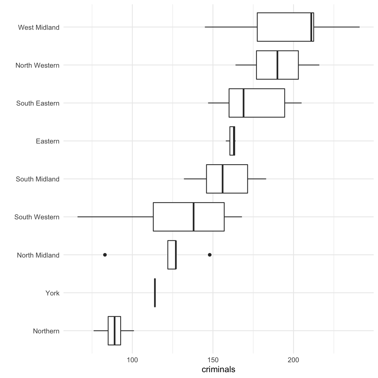
Let’s load the crimes data and look at the aggregated stats along with the distribution of criminals according to the region_name.

Now, let’s examine the density plots, scatterplots and correlation between public_houses and criminals.

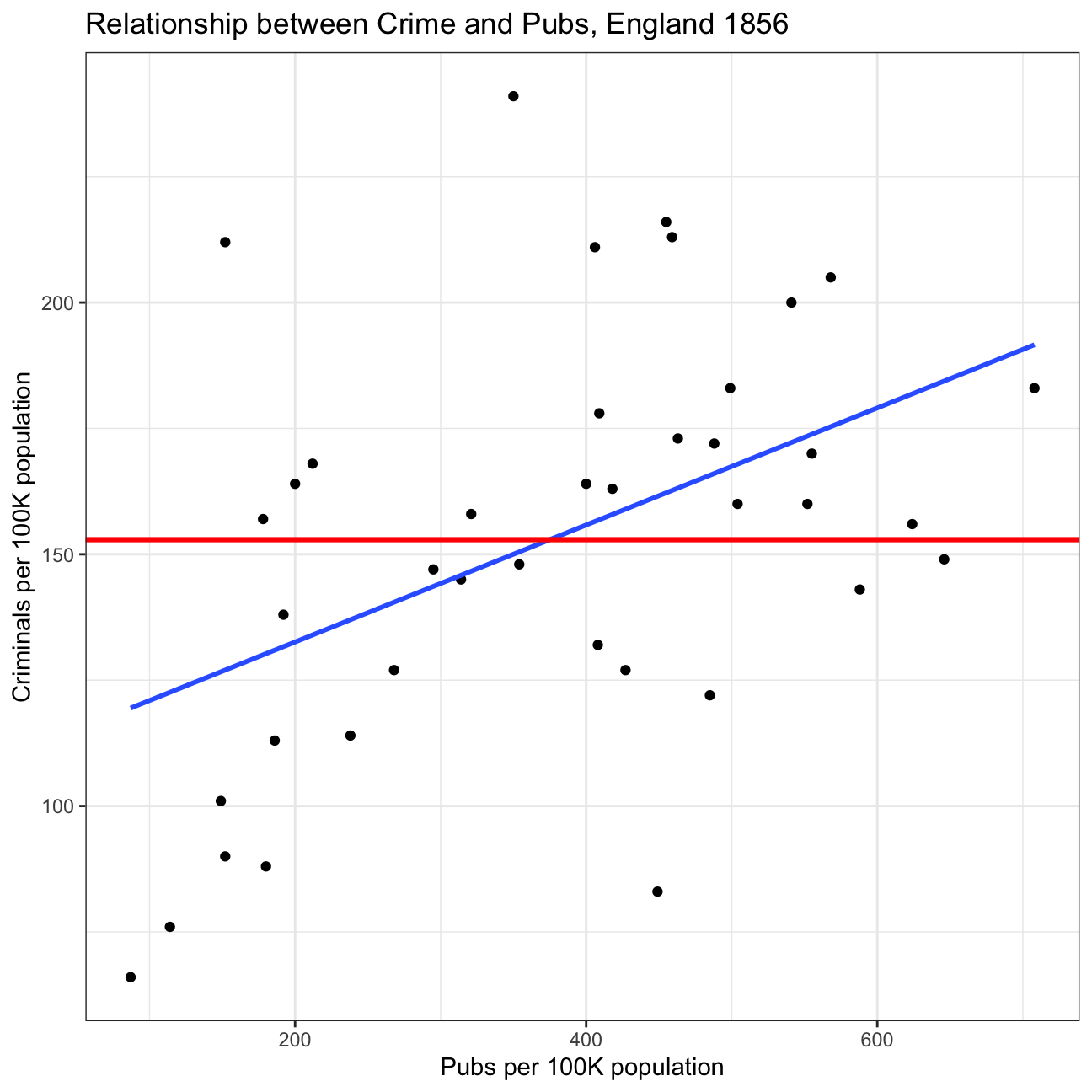
Using the different variables available to us, let’s create multiple models starting from base model of using mean value. The t-stat of each variable included and the adjusted R-square parameters will help in decided the appropriate model for our usecase.

term	estimate	std.error	statistic	p.value	conf.low	conf.high
(Intercept)	153	6.55	23.3	1.57e-24	140	166

term	estimate	std.error	statistic	p.value	conf.low	conf.high
(Intercept)	109	14.8	7.41	6.9e-09	79.5	139
public_houses	0.116	0.0361	3.22	0.00263	0.0431	0.189

term	estimate	std.error	statistic	p.value	conf.low	conf.high
(Intercept)	173	35.8	4.82	2.57e-05	100	246
public_houses	0.123	0.035	3.52	0.00118	0.0523	0.194
school_attendance	-0.101	0.0441	-2.3	0.0276	-0.19	-0.0118
worship_attendance	0.0393	0.0413	0.951	0.348	-0.0446	0.123

term	estimate	std.error	statistic	p.value	conf.low	conf.high
(Intercept)	179	35.2	5.07	1.12e-05	107	250
public_houses	0.126	0.0348	3.63	0.000854	0.0558	0.197
school_attendance	-0.0765	0.0356	-2.15	0.0381	-0.149	-0.00443

Let’s compare all these models to get a high level view on the best one.

Comparison of models
	(1)	(2)	(3)	(4)
(Intercept)	152.900	109.340	172.886	178.813
	(6.549)	(14.755)	(35.839)	(35.246)
public_houses		0.116	0.123	0.126
		(0.036)	(0.035)	(0.035)
school_attendance			-0.101	-0.077
			(0.044)	(0.036)
worship_attendance			0.039
			(0.041)
#observations	40	40	40	40
R squared	0.000	0.214	0.319	0.302
Adj. R Squared	0.000	0.194	0.262	0.264
Residual SE	41.416	37.193	35.583	35.536